GPU-accelerated Gibbs Sampler
Luofeng Liao
2019-09-05
intro.RmdMotivation
The Bayesian statistical paradigm is particular desirable in the big-data setting, because it allows us to impose prior knowledge on the data and produces a posterior distribution that summarizes knowledge from both data and humans. However, it is inherently computation-heavy. The advance of parallel computing sheds new light upon Bayesian inference. In (Lee et al. 2010) the author summarizes some efficient examples of parallel Bayesian methods. Inspired by this, this project implements the GPU version of the hierarchical models in (Makalic and Schmidt 2016), which features sparse estimates of the regression coefficients and is robust to non-Gaussian noise. The tremendous speed-up obtained by GPU shows the prospect of large-scale Bayesian inference.
Model Description
Bayesian inference is a “simple” trilogy:
- Specify priors;
- Based on likelihood, calculate the posterior;
- Sample from the posterior. Of course model checking is required for a specific data set.
The hierarchical Bayesian model proposed in Makalic and Schmidt (2016) is interesting in that it features continuous shrinkage prior densities and heavy-tailed error models. Formally, for responses \(z = \{z_1, \cdots, z_n \}\) and data matrix \(X = (x_1,\cdots, x_n)^T \in \mathbb{R}^{n \times p}\) of \(p\) predictors, we construct the following hierarchical model.

The model consists of two major components:
- the sampling distribution of the data, \(z\), and
- the prior distribution imposed on the regression coefficients \(\beta\).
The scale parameter \(\sigma^2\) is given the scale invariant prior \(\pi(\sigma^2) \propto 1/\sigma^2\), the intercept term \(\beta_0\) the uniform prior, and the global shrinkage parameter \(\tau\) the half-Cauchy distribution \(C^+(0,1)\), i.e., \(\pi(\tau) = 2/\pi(1+\tau^2),\tau>0\).
Below is an overview of the project.

Heavy-tailed error distributions
The scale parameter \(\sigma^2>0\) and the latent variables \(\{\omega_1,\cdots,\omega_n \}\) are used to model a variety of error distributions, that is, the distribution of \(e_i = z_i - \beta_0 - X_{i\cdot}\beta\) given all other variables.
As a reminder, we call \(Z\) follows a Gaussian scale mixture if it can be generated by \[Z|\lambda \sim \mathcal{N}(\mu,g(\lambda)\sigma^2), \lambda \sim \pi(\lambda)d\lambda.\] Different choices of \(\lambda\) and the mixing density \(g(\lambda)\) result in various non-Gaussian distributions of \(Z\).
In this project, we plan to provide the choices listed in the following table. Note \(\operatorname{E}\) is the exponential distribution, \(\operatorname{IG}\) is the inverse-Gamma distribution.
- \(\omega_i = 1\) , \(e_i\)’s are Gaussian errors (DONE)
- \(\omega_i \sim \operatorname{E}(1)\) , \(e_i\)’s are Laplace errors (DONE)
- \(\omega_i \sim \operatorname{IG}(\delta/2,\delta/2)\) , \(e_i\)’s are Student-\(t\) of df \(\delta > 2\) (TODO)
Sparsity-inducing priors
The hyperparameters \(\tau^2\) and \((\lambda_1,\cdots, \lambda_p)\) are used to model the sparsity in the coefficients and act as globa and local shrinkage. In other words, we care about the distribution of \(\beta\) given \(\tau^2\) and \((\lambda_1,\cdots, \lambda_p)\).
Currently our project provides the following three options in Tab.2. The Horseshoe estimator is relatively exotic. The general idea is to construct a prior on \(\beta\) that has an infinitely tall spike at 0 and heavy, Cauchy-like tails that decay like \(f(x)=1/x^2\).
- \(\lambda _ { j } ^ { 2 } = 1\), Ridge regression (TODO)
- \(\lambda _ { j } ^ { 2 } \sim \operatorname { E } ( 1 )\), The lasso (DONE)
- \(\lambda _ { j } \sim { C } ^ { + } ( 0,1 )\) , The Horseshoe estimator (TODO)
A Simulation Study
This part follows closely the simulation section of (Makalic and Schmidt 2016).
We construct a data set \(X \in \mathbb{R}^{ 50 \times 10}\) with \({Cov}(X_{\cdot i},X_{\cdot j}) = 0.5^{|i-j|}\) and \(\beta \in \mathbb{R}^{10}\) with only four non-zero entries. \(y_i = \beta_0 + X_{i\cdot}\beta + e_i\), where \(e_i\) is Laplace noise. Then we run both lasso (the left image) and the Bayesian regression with Laplace errors (the right one) and the Horseshoe type sparsity to discover the non-zero coefficients. The advantages of the model are (i) absence of hyperparameters and (ii) relatively more accurate estimates.

The Parallel Gibbs Sampler
One of the most commonly used methods to sample from the posterior distribution is the Gibbs sampler. To sample from a multivariate distribution, for example, \(f(x_1,x_2,x_3)\), we can sample from the following conditionals iteratively.
\[\begin{align} x_1^{k+1}\sim f_{1|2,3}(\cdot|x_2^k,x_3^k),\,\, x_2^{k+1} \sim f_{2|1,3}(\cdot|x_1^{k+1},x_3^k),\,\, x_3^{k+1} \sim f_{3|1,2}(\cdot|x_1^{k+1},x_2^{k+1}),\, \cdots \end{align}\]For example, the model with Student-\(t\) errors and \(\lambda _ { j } ^ { 2 } \sim \operatorname { E } ( 1 )\) has the following set of full conditionals (we suppress notations for “given all other variables”):
\[\begin{align} \beta &\sim \mathcal { N } _ { p } \left( \tilde { { \mu } } , { A } _ { p } ^ { - 1 } \right), 1/{\xi} \sim \operatorname{E}(1+{1}/{\tau^2}), 1/\nu_j \sim \operatorname{E}(1+{1}/{\lambda_j }) \\ \omega_i^2 &\sim \mathrm { IG } \big( \frac { \delta + 1 } { 2 } , \frac { 1 } { 2 } ( { e _ { i } ^ { 2 } } / { \sigma ^ { 2 } } + \delta ) \big) , \lambda_j \sim \operatorname{E}( { 1 }/ { \nu _ { j } } + { \beta _ { j } ^ { 2 } }/ { 2 \tau ^ { 2 } \sigma ^ { 2 } }) \\ \sigma^2 &\sim \mathrm { IG } \big( \frac { n + p } { 2 } , \frac { 1 } { 2 } ( \sum _ { i = 1 } ^ { n } { e _ { i } ^ { 2 } }/ { \omega _ { i } ^ { 2 } } + \sum _ { j = 1 } ^ { p } { \beta _ { j } ^ { 2 } } / { \tau ^ { 2 } \lambda _ { j } ^ { 2 } } ) \big), \\ \tau^2 &\sim \operatorname{IG}(\frac{p+1}{2}, { 1 }/ { \xi } + \frac { 1 } { 2 \sigma ^ { 2 } } \sum _ { j = 1 } ^ { p } { \beta _ { j } ^ { 2 } } / { \lambda _ { j } ^ { 2 } }) \end{align}\]where \(j = 1,\cdots,n,i = 1,\cdots, p\). \(\xi\) and \(\nu_j\) are auxiliary variables.
Conditional independence in the posterior distributions
We \(x\) and \(y\) are conditionally independent given \(z\) if \(p(x,y|z) = p(x|z)p(y|z)\). In the above conditionals, variables listed in the same line are conditionally independent, and therefore can be sampled simultaneously. See Fig.3 for demostration. This is particularly important in the big-data scenario. For large \(n\) and \(p\), sampling sequentially for \(\nu_j,\lambda_j,\omega_i\) would be expensive.
Thd following graph illustrates the sampling schemes. From top to bottom are the streams for sampling and collecting \((\beta,\xi,\nu)\), \((\omega,\lambda)\), \(\sigma\), \(\tau\) and finally an independent stream generating a lot of uniforms.

GPU and CUDA
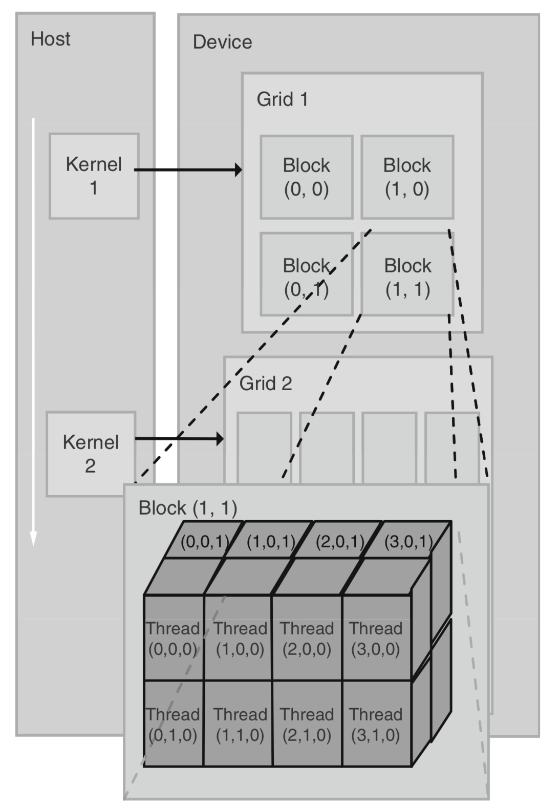
GPU is well suited for SIMD (Single Instruction Multiple Data) parallelization, i.e., tasks that can be partitioned into many parts and there is little dependence across sub-tasks. In CUDA terminology, when we start a task (summing two matrices, for example), we launch a , and and (Fig. 4) determine the way we partition the task. See the following graph (Kirk and Wen-Mei 2016).
The following techniques are crucial in the sampling from the posterior:
cuBLAS: parallel linear algebra subroutines. Sampling from high-D Gaussian is the very bottle-neck of the algorithm, because we need to draw a vector from a \(p\)-dimensional Gaussian that changes at every iteration. Most techniques that I know of are based on matrix factorization, e.g., Cholesky, QR or SVD. This can be done in parallel using the well-tuned CUDA package cuBLAS.
Streaming. Streaming allows us to execute multiple kernels at the same time, if GPU resources allow. (a) We launch multiple threads to sample \(\nu_1,\cdots, \nu_p\), and launch multiple kernels to sample \(\beta,\xi,\nu\) in parallel. (b) Generate uniforms concurrently. Many sampling methods in the model are inverse transformation. We can first pre-generate lots of uniforms, and then refill it when it is used up. All these can be done concurrently with the sampling.
Asynchronous data transfer. We can execute the program and transfer data back to CPU at the same time. This can be applied in gathering draws from the posterior while keep the sampler running. Due to the expense of CPU-GPU data transfer, this could save a lot time.
Thrust: building-block parallel algorithms. Thrust is a CUDA library that provides the parallel version of C++ Standard Template Library (STL). Moreover, Thrust provides a rich collection of data parallel primitives such as transformation, reduction, scanning and sort.
The CUDA memory model. CUDA has a wide variety of memory types, differing in their scope, sizes, latency and access pattern. Careful manipulation of memory is key to successful parallel programs. For example. is only available to threads in the same block, and it is very fast because it is on-chip. On the other hand, the size of shared memory is very limited: at most 64 KB (this is configurable during runtime). Other advanced memory managing techniques include pinned memory, zero-copy memory and so on.
How Fast Is It?
To demonstrate the advantage to GPU-accelerated Gibbs sampler, I compare the MATLAB implementation Makalic and Schmidt (2016) and my implementation using CUDA. My code is run on a Nvidia Tesla P100 with 3584 CUDA cores and 16 GB GPU memory. The MATLAB implementation is run on my Macbook pro with 3.1 GHz Intel Core i5 and 16GB memory. We can see in all cases CUDA code outperforms the MATLAB implementation, and the advantage becomes increasingly prominent as the data size grows. Each experiment runs for 5000 iterations, from a model with Horseshoe-type sparsity and Gaussian noise.
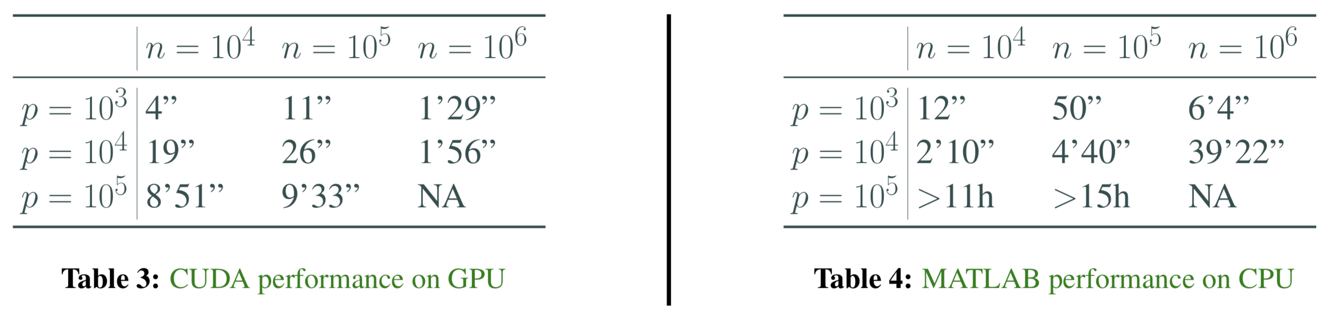
We should also note that, despite exciting results, GPU could not handle super-large datasets due to memory limitation.
Future Work
Asynchronous Gibbs sampler suits GPU much better (\(x_i^{k+1}\sim f_{i|others}(\cdot|x_1^k,\cdots,x_p^k),\forall i\)), but it requires theoretical justifications.
Deploy the code across multiple GPUs. For example, a data set of \(n = 1,000,000\) and \(p = 10,000\), which takes about 40 GB RAM, already well exceeds the capacity of GPU.
Acknowledgement
Thank Dr. Enes Makalic from University of Melbourne for the idea of the project. Thank Google Cloud Platform (GCP) for free education credits to cloud computing service. Finally a huge thankyou to Nvidia engineers for bringing these amazing toys to our world.
Liao acknowledges the support of XiYuan Undergraduate Academic Program of Fudan University. The project is awarded the Runnerup Award out of around 30 equally competitive posters in the student poster section of 2018 Fudan Science and Innovation Forum.
References
Kirk, David B, and W Hwu Wen-Mei. 2016. Programming Massively Parallel Processors: A Hands-on Approach. Morgan kaufmann.
Lee, Anthony, Christopher Yau, Michael B Giles, Arnaud Doucet, and Christopher C Holmes. 2010. “On the Utility of Graphics Cards to Perform Massively Parallel Simulation of Advanced Monte Carlo Methods.” Journal of Computational and Graphical Statistics 19 (4). Taylor & Francis: 769–89.
Makalic, Enes, and Daniel F Schmidt. 2016. “High-Dimensional Bayesian Regularised Regression with the Bayesreg Package.” arXiv Preprint arXiv:1611.06649.